STAT 440/540: Data analysis example using techniques from Chapter 3

The data set we consider is the time-to-failure in minutes of 50 electrical components. Each component was manufactured using a ratio of two types of materials; this ratio was fixed at 0.1, 0.2, 0.3, 0.4, and 0.5. Ten components were observed to fail at each of these manufacturing ratios in a designed experiment. It is of interest to stochastically model the failure-time as a function of the ratio, to determine if a significant relationship exists, and if so to describe the relationship simply.

We start from the point of having the data loaded into Minitab worksheet columns labeled x and y. A scatterplot is obtained by choosing “Graph” and “Plot…” and by picking the appropriate x and y variables and clicking “OK.” The standard assumptions of linear mean function and constant variance in the model Y_i = b₀ + b₁ X_i + e_i with the e_i ~ N(0, s²) are immediately suspect:

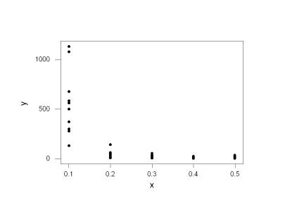
The error variance decreases as the predictor values increase and we can use the Breusch-Pagan test to formally test the constant variance assumption. Recall that this test assumes the full model Y_i = b₀ + b₁ X_i + e_i, where the e_i are independent normal random variables with mean zero and variance exp(g₀ + g₁ X_i). We test H₀: g₁ = 0 in this model as follows. We click on the “Session” window and then check “Enable Commands” under “Editor.” We can now type in Minitab commands directly. First we regress y on x, note the SSE, and store the raw residuals. We need the sum of squares regression, SSR*, from regressing the raw squared residuals (e_i)² (from our fit of the standard regression model) versus the X_i. The test statistic is given by (SSE*/2) / (SSE/n)² and has an approximate X² with 1 df when the null hypothesis holds. See page 115 for more detail. Here we regress y on x and store the raw residuals in a column called raw:

MTB > name c6 'raw' c7 'rawSQ'

MTB > regress y 1 x;

SUBC> residuals raw.

Analysis of Variance

Source DF SS MS F P

Regression 1 1279453 1279453 29.88 0.000

Residual Error 48 2055067 42814

Total 49 3334520

Now we regress the squared raw residuals on x and note the SSR*:

MTB > let rawSQ = raw**2

MTB > regress rawSQ 1 x.

Analysis of Variance

Source DF SS MS F P

Regression 1 89123428186 89123428186 8.50 0.005

Residual Error 48 5.03351E+11 10486480769

Total 49 5.92475E+11

Here we assign the constant k1 to be the Bruesch-Pagan test statistic, find k2 = P(X² £ k1) and take k3 = P(X² > k1), the p-value for the test:

MTB > let k1 = (89123428186/2)/((2055067/50)**2)

MTB > CDF k1 k2;

SUBC> ChiSquare 1.

MTB > let k3 = 1 - k2

MTB > print k3

K3 0.000000281

The p-value for this test is zero to 6 decimal places and we have extremely strong evidence of non-constant variance assuming other assumptions are met (they’re not; linear mean structure is obviously questionable here too, but we’ve got to start someplace.)

A transformation of x alone will not help the non-constant variance and we’ll concentrate on a power transformation of y first. Of the prototype plots on page 130, this data somewhat resembles figure 3.15 (b). We might try any one of the three suggested transformations of y, but will first try Atkinson’s constructed variable test for some guidance. The following constructs Atkinson’s variable and performs the test; the relevant output follows:

MTB > name c3 'w'

MTB > let w = y*(loge(y)-mean(loge(y))-1)

MTB > regress y 2 x w

Predictor Coef SE Coef T P

Constant 125.57 14.41 8.71 0.000

x -249.14 41.26 -6.04 0.000

w 0.372809 0.009234 40.38 0.000

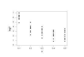
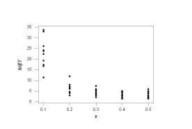
The p-value for testing H₀: b₂ = 0 in the model Y_i = b₀ + b₁ X_i + b₂ W_i + e_i, and equivalently H₀: r = 1 in the model (Y_i)^r = b₀ + b₁ X_i + e_i, is 0.000, providing strong evidence that a power transformation will be useful. The estimated power is 1 – 0.37 = 0.63, which is approximately equal to 0.5. Based on the scatterplot above, we might try using log(Y_i) or (Y_i)^0.5 as response variables. Let’s look at these responses versus the X_i’s.

MTB > name c4 'sqtY' c5 'logY'

MTB > let sqtY = sqrt(y)

MTB > let logY = log(Y)

Now plot them using the “Graph” pull-down menu. You will see the following commands appear in the session window, in case you want to do all of this by hand:

MTB > Plot 'sqtY'*'x' 'logY'*'x';

SUBC> Symbol;

SUBC> ScFrame;

SUBC> ScAnnotation.

The plots show that the log-transformation has mitigated the non-constant variance but the square-root-transformation did not (a plot of (Y_i)^-1 versus X_i shows dramatically increasing variance):

Let’s regress the log-transformed Y_i’s onto the X_i’s. There are repeated observations at the predictor values and there appears to be some curvature to this plot, so we will also perform the pure-error lack of fit test.

MTB > regress logY 1 x;

SUBC> pure.

Analysis of Variance

Source DF SS MS F P

Regression 1 82.721 82.721 81.53 0.000

Residual Error 48 48.699 1.015

Lack of Fit 3 21.714 7.238 12.07 0.000

Pure Error 45 26.985 0.600

Total 49 131.419

We obtain the following test statistic F* = [(SSE(R) -SSE(F))/(dfE(R)-dfE(F))] / MSE(F) = [21.714/3] / 0.600 = 12.07 and there is a corresponding p-value of 0.000 for the null hypothesis

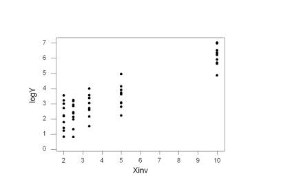
H₀: E{ log(Y_i) } = b₀ + b₁ X_i, i.e. that a line is appropriate. From the prototypical plots on page 127, we will try the inverse-transformation in the manufacturing ratio: (X_i)^-1. First we define the reciprocal of x:

MTB > name c8 'Xinv'

MTB > let Xinv = 1/x

A scatterplot of log(Y_i) versus (X_i)^-1 shows drastic improvement:

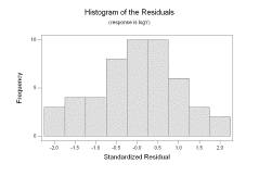
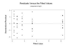
We regress log(Y_i) onto (X_i)^-1, save the studentized residuals, and present several diagnostic plots. Under “Stat” choose “Regression” and then “Regression…” again. As the “Response:” choose logY and as the “Predictors:” choose Xinv. Click the “Graphs…” button, choose “Standardized” residuals and choose to display a “Histogram of residuals” and the “Residuals versus fits,” and click “OK.” Click “Options…” and click the “Pure error” Lack of Fit Test and click “OK.” Click “Storage…” and choose to store the “Standardized residuals” and the “Fits” in columns and click “OK.” Click “OK” again and we have the following output:

Regression Analysis: logY versus Xinv

The regression equation is

logY = 1.15 + 0.497 Xinv

Predictor Coef SE Coef T P

Constant 1.1537 0.1990 5.80 0.000

Xinv 0.49732 0.03677 13.52 0.000

S = 0.7544 R-Sq = 79.2% R-Sq(adj) = 78.8%

Analysis of Variance

Source DF SS MS F P

Regression 1 104.10 104.10 182.89 0.000

Residual Error 48 27.32 0.57

Lack of Fit 3 0.34 0.11 0.19 0.905

Pure Error 45 26.98 0.60

Total 49 131.42

Unusual Observations

Obs Xinv logY Fit SE Fit Residual St Resid

19 2.5 0.807 2.397 0.131 -1.590 -2.14R

R denotes an observation with a large standardized residual

Note that Minitab flags observations that have a studentized residual unusually large in magnitude. These observations are potential outliers, points not fit well by the model. You can see observation 19 on the previous scatterplot at the bottom of the cluster of points at 1 / X₁₉ = 2.5.

The pure-error lack of fit test yields the following results: SSLOF=SSE(R)-SSE(F)=0.34. dfLOF = dfE(R) – dfE(F) = 5 – 2 = 3. MSLOF = SSLOF / dfLOF = 0.34 / 3. This statistic has an F(dfLOF, dfE(F)) distribution when the mean is a line.

We have highly significant regression parameters and 79.2% of the variability in logY is explained by Xinv. The p-value 0.905 indicates no lack of fit, and the histogram of standardized residuals and standardized residuals versus the fitted values show no evidence on non-normality, non-constant variance, or a pattern of over or under fitting:

The standardized residuals were saved in a column labeled SRES1; we perform the Ryan-Joiner normality test on them (under “Stat”, “Basic Statistics”, and “Normality Test…”) and obtain the following output:

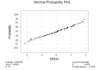
We see the resulting p-value is larger than 0.1. By comparison, the Anderson-Darling test yields a p-value of 0.733 and the Kolmogorov-Smirnov test yields a p-value larger than 0.15. All three tests don’t reject the null hypothesis that the standardized residuals came from a normal distribution. Simply to demonstrate how one would perform the modified Levene test in this circumstance, look at the standardized residuals versus the fitted values above. The plot looks fine, but we may detect a slight decrease in variance for residuals corresponding to fitted values larger than 3. We create an index separating the residuals into groups corresponding to fits larger than 3 and fits smaller than 3 in the following manner, assuming that the fitted values were saved in a column labeled FITS1:

MTB > Name C11 = 'Group'

MTB > Let 'Group' = Sign(FITS1-3)

This places a “1” under Group when a fitted value is larger than 3 and a “-1” otherwise. Under “Stat” we pick “ANOVA” and then “Test for Equal Variances…” Choose SRES1 as the “Response:” and Group as the “Factors:” and click “OK.” We see the following:

Test for Equal Variances

Response SRES1

Factors Group

ConfLvl 95.0000

Levene's Test (any continuous distribution)

Test Statistic: 0.520

P-Value : 0.474

The p-value for the hypothesis that the population variances in the two groups are equal is 0.474. We accept they are equal.

Finally, we wish to convert our statistical model back into the original units.

The median survival time as a function of the covariates is estimated to be

Med{ Y } @ exp( 1.15 + 0.497 / X ).

Why? Remember the model is log(Y) = b₀ + b₁ / X + e where e ~ N(0, s²). We have P(e < 0) =0.5 and thus P( Y < exp(b₀ + b₁ / X) ) = P( exp(b₀ + b₁ / X + e) < exp(b₀ + b₁ / X) ) = P( exp(b₀ + b₁ / X ) exp (e) < exp(b₀ + b₁ / X) ) = P(exp (e) < 1 ) = P(e < 0 ) =0.5. We can also obtain prediction intervals, for example when X = 0.3:

MTB > regress logY 1 Xinv;

SUBC> pred 3.33.

Predicted Values for New Observations

New Obs Fit SE Fit 95.0% CI 95.0% PI

1 2.810 0.116 ( 2.577, 3.043) ( 1.275, 4.345)

The prediction interval is then ( exp(1.275), exp(4.345) ) = ( 3.58, 77.09 ) minutes. The estimated median survival time at this ratio is exp( 2.81 ) = 16.6 minutes.