GLM Application in Spark: a case study
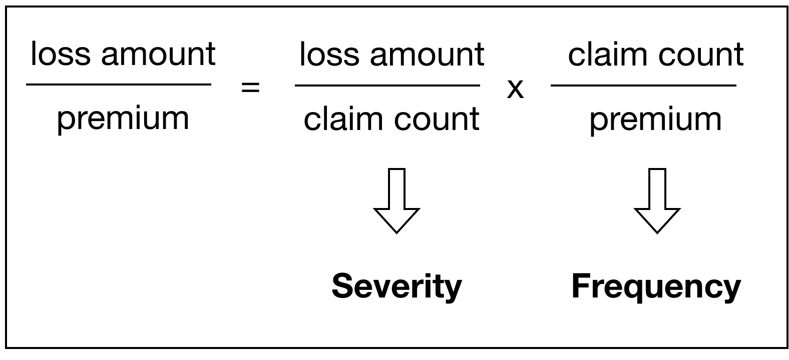
In the insurance industry, one important topic is to model the loss ratio, i.e, the claim amount over the premium. GLM is a popular method for its interpretability. Plus, regulators like it because they do not want to learn new stuff. Within this framework, there is a lot that we can do. For instance, one have to decide from tweedie model and the frequency severity model. We'll emphasize the latter one in this article, but let's take a look at tweedie first.
The tweedie model
A well established way is to use tweedie distribution as the underlying in glm to predict the loss ratio. This distribution is a mixture of poisson and gamma distribution. To be specific, there is a non-zero probability at 0, and taking that point mass off, the remaining is a gamma distribution. This is to reflect the fact that most of the policies got zero claims at the end of the year.
The problem of this process is a lack of understanding of frequencies. Consider the following two scenarios:
- Client A got 10 claims, 100 dollars each in the last year.
- Client B got only 1 claim but with 1000 dollars in the last year.
The tweedie model thinks these two are identical since the response variable does not include frequencies whatsoever. In fact, sometimes we do not care about the difference, but sometimes we do. This is the rationale for frequency-severity model.
The frequency severity model
An overview
The frequency severity model, on the other hand, allows us to model the frequency explicitly. As you might have guessed, this is more like a two stage model, both of which are based on glm framework, and the following graph gives an oversimplified way to demonstrate this. We'll elaborate the model setups in a minute.

This scheme has more flexibility--we can do variable selection independently, which might lead to some interesting findings. For instance, you may realize that some factors have an impact on one process but not another. Here is a fun fact. In the severity model, the insurance company usually pays much more when there is an attorney present. So get a lawyer.
In terms of performance, there is no clear winner. Sometimes the frequency-severity model yields better results, sometimes it does not. In this case, we are given the dataset and selected variables, and will apply the frequency-severity framework and see if we can beat tweedie.
Data Preprocessing
The first part is pretty standard. We simply impute all missing values in the data set, with numerical types filled by sample mean while string types filled by a new category called "missing". Since this script is supposed to run on a Spark 2.1 version, we used the old way instead of Imputer function.
df = sqlContext.read.format('com.databricks.spark.csv')\
                    .option('header', 'true')\
                    .option('inferschema', 'true')\
                    .load("hdfs://TDHFD6/user/hl89372/GLM_DATA.csv")

from collections import defaultdict

data_types = defaultdict(list)
for entry in df.schema.fields:
    data_types[str(entry.dataType)].append(entry.name)

strings = data_types["StringType"]

missing_data_fill = {}
for var in strings:
  missing_data_fill[var] = "missing"
df = df.fillna(missing_data_fill)

numericals = data_types["DoubleType"] + data_types["IntegerType"] \
                                      + data_types["LongType"]

mean_dict = { col: 'mean' for col in numericals}
col_avgs = df.agg( mean_dict ).collect()[0].asDict()
col_avgs = { k[4:-1]: v for k,v in col_avgs.iteritems() }
df = df.fillna(col_avgs)
Good news is we do not have to do variables selection since somebody else has taken care of it. The variable has been store in a variables called variable_list_emblem.
response_vars = ["LT_INDEM_ULT_WITH_EXCSS_AMT",
                 "LT_MED_ULT_WITH_EXCSS_AMT",
                 "MO_MED_ULT_WITH_EXCSS_AMT",
                 "LT_INC_INDEM_CLM_CNT",
                 "MO_INC_MED_CLM_CNT"]

df = df.select(response_vars + variable_list_emblem)
On the other hand, there's something that needs to be done for the response variables.
- Rename some variables in a more friendly way. Renaming or create alias is incredibly important if you work with the hard-to-remember acronyms all day. Trust me. Rename it in a more friendly way.
- I need to create some new columns. For instance, the real severity of indemnity is the sum of
LT_INDEM_ULT_WITH_EXCSS_AMTandLT_MED_ULT_WITH_EXCSS_AMT, in which the first variable reflects the loss from not being able to work any longer and the second variables reflects the medical expenses. - Besides, I need to get the inverse of claim counts since I need them for the weights in GLM. More on that later.
df = df.withColumnRenamed("MO_MED_ULT_WITH_EXCSS_AMT", "medical_amount")
df = df.withColumnRenamed("MO_INC_MED_CLM_CNT", "medical_count")
df = df.withColumnRenamed("LT_INC_INDEM_CLM_CNT", "indemnity_count")

df = df.withColumn("indemnity_amount", df["LT_INDEM_ULT_WITH_EXCSS_AMT"] + df["LT_MED_ULT_WITH_EXCSS_AMT"])
df = df.withColumn("medical_ratio", df["medical_amount"]/df["medical_count"])
df = df.withColumn("indemnity_ratio", df["indemnity_amount"]/df["indemnity_count"])

df = df.withColumn("inverse_medical_count", 1/df["medical_count"])
df = df.withColumn("inverse_indemnity_count", 1/df["indemnity_count"])
Note that you have to use the equal sign to assign the renamed data frame back to df, otherwise your column will not be renamed. This somehow reminds me of the drop method in pandas. I do not think this is nice design, but anyways.
Since we deal with strings and numbers separately, two pipelines are used. For strings, we use OneHotEncoder and StringIndexer to convert them into levels; for numbers we scaled and normalized them. A fun fact about pipeline is this: even though all components in the pipeline do not have the fit method and only got transform, you still have to do .fit(df).transform(df) when using a pipeline.
from pyspark.ml import Pipeline
from pyspark.ml.feature import OneHotEncoder, StringIndexer, VectorAssembler

strings = [var for var in variable_list_emblem if var in data_types["StringType"]]
stage_string = [StringIndexer(inputCol= c, outputCol= c+"_string_encoded") for c in strings]
stage_one_hot = [OneHotEncoder(inputCol= c+"_string_encoded", outputCol= c+ "_one_hot") for c in strings]

ppl = Pipeline(stages= stage_string + stage_one_hot)
df = ppl.fit(df).transform(df)

from pyspark.ml.feature import Normalizer, VectorAssembler, StandardScaler

numericals = [var for var in variable_list_emblem if var not in data_types["StringType"]]
numericals_out = [var+ "_normalized" for var in numericals]

vs = VectorAssembler(inputCols= numericals, outputCol= "numericals")
df = vs.transform(df)

scaler = StandardScaler(inputCol = "numericals", outputCol = "numericals_after_scale")
normalizer = Normalizer(inputCol = "numericals_after_scale", outputCol= "normalized_numericals", p=1.0)

ppl2 = Pipeline(stages= [scaler, normalizer])
df = ppl2.fit(df).transform(df)
Training the GLM model
Let's finally put them together and split them into training set and test set.
categoricals = [var for var in df.columns if var.endswith("_one_hot")]
num = ["numericals"]
vector_assembler = VectorAssembler(inputCols= categoricals + num, outputCol= "features")
df = vector_assembler.transform(df)

training_set, test_set = df.randomSplit([0.7, 0.3], seed = 2017)
Note that in this case, we made it more complex by modeling the medical expenses and the indemnity expenses separately, since these two variables have different behavior. For the frequency model, we adopted the most popular setup, using premium as weights and poisson as the underlying distribution.
frequency_medical =  GeneralizedLinearRegression(family="poisson",
                                           link="log",
                                           maxIter=10,
                                           fitIntercept = True,
                                           labelCol = "medical_count",
                                           weightCol = "mdl_base_co_ep_amt",
                                           regParam=0.3)


frequency_indemnity =  GeneralizedLinearRegression(family="poisson",
                                           link="log",
                                           maxIter=10,
                                           fitIntercept = True,
                                           labelCol = "indemnity_count",
                                           weightCol = "mdl_base_co_ep_amt",
                                           regParam=0.3)

frequency_medical.setPredictionCol("prediction_severity_medical")
frequency_indemnity.setPredictionCol("prediction_frequency_indemnity")
Note that I used.setPredictionCol("prediction_frequency_indem") to give the prediction column a customized name. This is because I want to append all four columns of predictions from four models into one data frame and doing this can avoid naming collision. Otherwise you'll see something like prediction column already exists.
The setup of the second stage model (severity model) comes from Prediction Modelling Appication in Actuarial Science. We use gamma as underlying distribution and inversed claim accounts as weights. It looks like this.
severity_indem =  GeneralizedLinearRegression(family="gamma",
                                           link="log",
                                           maxIter=10,
                                           labelCol = "indemnity_ratio",
                                           weightCol = "inverse_indemnity_count",
                                           fitIntercept = True,
                                           regParam=0.3)

severity_medical =  GeneralizedLinearRegression(family="gamma",
                                           link="log",
                                           maxIter=10,
                                           labelCol = "medical_ratio",
                                           weightCol = "inverse_medical_count",
                                           fitIntercept = True,
                                           regParam=0.3)

severity_indem.setPredictionCol("prediction_severity_indem")
severity_medical.setPredictionCol("prediction_severity_medical")
Tuning regularization parameters
However, it seems arbitrary to assume regParam=0.3 in all four cases. It is a better idea to do a grid search. Here is how to implement this for medical frequency model. You have to specify the candidates you want to search, and the metrics to evaluate the regressor.
from pyspark.ml.tuning import ParamGridBuilder, CrossValidator
from pyspark.ml.regression import GeneralizedLinearRegression, GBTRegressor
from pyspark.ml.evaluation import RegressionEvaluator

frequency_medical =  GeneralizedLinearRegression(family="poisson",
                                           link="log",
                                           maxIter=10,
                                           fitIntercept = True,
                                           labelCol = "medical_count",
                                           weightCol = "mdl_base_co_ep_amt",
                                           regParam=0.3)
para_grid = ParamGridBuilder()\
           .addGrid(frequency_medical.regParam, [0.1, 0.3, 0.5, 0.7, 0.9])\
           .build()

evaluator = RegressionEvaluator(labelCol="medical_count",
                                predictionCol="prediction",
                                metricName="rmse")
cross_val = CrossValidator(estimator = frequency_medical,
                           estimatorParamMaps= para_grid,
                           evaluator = evaluator)

model_frequency_medical = cross_val.fit(trainining_set)
Remember that we actually got four models: frequency of medical claim, frequency of indemnity claim, severity of indemnity claim and severity of medical claim. The setup of these models are actually pretty similar to each other. To avoid repeating ourselves four times, we write a function to do this. The model-specific info is stored in the dictionaries.
One nuance here: we run the frequency model on full dataset, but run severity model only on those with at least more than on claim. Spark got a very elegant way to do this and it works exactly as expected if you are familiar with SQL.
from pyspark.ml.tuning import ParamGridBuilder, CrossValidator
from pyspark.ml.regression import GeneralizedLinearRegression, GBTRegressor
from pyspark.ml.evaluation import RegressionEvaluator

info_frequency_medical = {"labelCol": "medical_count",
                          "weightCol": "mdl_base_co_ep_amt",
                          "family": "poisson" }

info_severity_medical = {"labelCol": "medical_ratio",
                         "weightCol": "inverse_medical_count",
                         "family": "gamma" }

info_frequency_indem = {"labelCol": "indemnity_count",
                        "weightCol": "mdl_base_co_ep_amt",
                        "family": "poisson" }

info_severity_indem = {"labelCol": "indemnity_ratio",
                       "weightCol": "inverse_indemnity_count",
                       "family": "gamma" }

training_set_for_medical = training_set.where((training_set["medical_amount"] > 0) & (training_set["medical_count"] > 0))
training_set_for_indmnity = training_set.where((training_set["indemnity_amount"] > 0) & (training_set["indemnity_count"] > 0))


def cross_valiation_maker(model_info, param_grid):
    #trainining_set, test_set = df.randomSplit([0.7, 0.3], seed = 2017)
    model =  GeneralizedLinearRegression(link="log", fitIntercept = True, maxIter= 10)

    model.setFamily(model_info["family"])
    model.setLabelCol(model_info["labelCol"])
    model.setWeightCol(model_info["weightCol"])

    model.setPredictionCol("prediction_" + model_info["labelCol"] )

    para_grid = ParamGridBuilder()\
           .addGrid(model.regParam, param_grid)\
           .build()


    evaluator = RegressionEvaluator(labelCol= model_info["labelCol"],
                                    predictionCol= "prediction_" + model_info["labelCol"] ,
                                    metricName="rmse")

    cross_val = CrossValidator(estimator = model,
                               estimatorParamMaps = para_grid,
                               evaluator = evaluator,
                               numFolds= 3 )

    if model_info["labelCol"] == "medical_ratio":
        training_set = training_set_for_medical

    if model_info["labelCol"] == "indemnity_ratio":
        training_set = training_set_for_indmnity

    fitted_model = cross_val.fit(training_set)

    return(fitted_model)
This is how to use the cross_validation_maker: there's two arguments: the first is the model information, which expects a dictionary, and the second is a list of penalization/regularization parameters to try out. Bear in mind that for each of candidates, we do a 3 fold cross validation, and thus this process will take much longer if we run it on the full data set. The returned object is the fitted model with training data, which can be used to make prediction directly.
model_freq_indem = cross_valiation_maker(info_frequency_indem, [0, 0.1,  0.3,  0.5])
model_freq_medical = cross_valiation_maker(info_frequency_medical, [0, 0.1,  0.3,  0.5])

model_severity_indem = cross_valiation_maker(info_severity_indem, [0, 0.1,  0.3,  0.5])
model_severity_medical = cross_valiation_maker(info_severity_medical, [0, 0.1,  0.3,  0.5])

df_predictions = model_freq_med.transform(test_set)
df_predictions = model_freq_indem.transform(df_predictions)

df_predictions = model_severity_medical.transform(df_predictions)
df_predictions = model_severity_indem.transform(df_predictions)
To recap, the four predictions are in the same data frame named df_predictions, with pre-defined name "prediction_severity_indem", "prediction_severity_medical", "prediction_frequency_medical", and "prediction_frequency_indem",from which we can derive the ultimate prediction, which is
df_predictions["prediction_severity_indem"]*df_predictions["prediction_frequency_indem"] +df_predictions["prediction_frequency_medical"]*df_predictions["prediction_frequency_medical"]
Based on which, we can create a new column prediction with another column target, which is the observed value.
df_predictions = df_predictions.withColumn("target", df["medical_amount"] + df["indemnity_amount"] )
df_predictions = df_predictions.withColumn("prediction", df_predictions["prediction_severity_indem"]*df_predictions["prediction_frequency_indem"]  + df_predictions["prediction_frequency_medical"]*df_predictions["prediction_frequency_medical"])
A User Defined Function (UDF) showcase
We'll next modify predictions from the frequency model. This is because the poisson regression usually gives fractions instead of integers in prediction. This is not a big issue generally, but since our model has a second stage, which might signify this issue.
For instance, if you got 0.01 in frequency model but got 100,000 in the severity model, you will still end up with 1000 as a prediction after combining the second stage. However, in reality this case should probably be 0 since 0.01 is close enough to be a claim free scenario. With that in mind, we force all predictions smaller than 0.01 to be 0. Of course you can tune this hyper-parameter later.
There is a perfect tool to do this in Spark--UDF: udf--user defined function. The logic is to first write a customized function for each element in a column, define it as udf, and apply it to the data frame. Udf usually has inferior performance than the built in method since it works on RDDs directly but the flexibility makes it totally worth it. And RDD is not that slow after all.
from pyspark.sql.types import DoubleType
from pyspark.sql.functions import udf

def shut_down_device(r):
    if r < 0.1:
        return 0.0
    else:
        return r

udf_sd = udf(shut_down_device, DoubleType())

df_predictions = df_predictions.withColumn("truncated_medical_count", udf_sd(df_predictions["prediction_frequency_medical"]))
df_predictions = df_predictions.withColumn("truncated_indemnity_count", udf_sd(df_predictions["prediction_frequency_indem"]))

df_predictions = df_predictions.withColumn("prediction", df_predictions["prediction_severity_indem"]*df_predictions["truncated_indemnity_count"] \
                          + df_predictions["prediction_frequency_medical"]*df_predictions["truncated_medical_count"])
Benchmarking
Here are two ways of calculating metrics. Spark-native strategy is to use RegressionEvaluator, which asks for the prediction column and observed real value, along with the metric. It's faster since it's a native function but the metrics are limited since the library is still young. We can also consider sklearn.metrics, which has got a wider range of tools but takes longer to run since serialization happens under the hood.
from pyspark.ml.evaluation import RegressionEvaluator
evaluator = RegressionEvaluator(
    labelCol="target", predictionCol="prediction", metricName="rmse")
rmse = evaluator.evaluate(df_predictions)
print("Root Mean Squared Error (RMSE) on test data = %g" % rmse)

from sklearn.metrics import r2_score
prediction_to_pandas = df_predictions.select(["prediction","target"]).toPandas()
r2 = r2_score(prediction_to_pandas.prediction, prediction_to_pandas.target)
print("R-square on test data = %g" % r2)
I hate to admit this but in this scenario, the tweedie model is actually better in terms of both R square and gini metric. The new model is like 10% worse in most of metrics. By the way, fitting all four models takes like 5min 41s on the server, which is pretty amazing considering the size of data (around half a million).
Q&A
Why we predict the claim amount in the end instead of loss ratio?
At least in our case the premium can be considered as a constant. It is called manually premium, which can be pre-determined based on risk scores and whatnot. We can always pull that number from external sources. This makes it more of a constant/multiplier thing rather than a random variable. So arguably, modeling the loss and modeling the loss ratio is equivalent in this case.
Can I use offset instead of weight?
Not actually. For one thing, Spark does not support the offset option; for another, adjusting offset is not equivalent in some cases (especially gamma distribution) to adjusting weights.Let me elaborate this. Let's say we want to rule out the impact of time in a Poisson regression in that ache monkey hunting example. We can do this by either use time as weights AND divide response variable by time or just use time as offsets. They are equivalent and you can do them exchangeably.
We can do this simply because the mean equals the variance of poisson distribution! In other cases, they are not. For instance, in a gamma distribution, if you divide mean by \(\lambda\), then the variance shrinks by \(\lambda^2\), which is not equivalent to adjusting weights any more.
After all, they sound similar but means different things. Offsets means "I don't want to consider that factor at all. Let's figure out a way to remove it" while weights means "the observations with more weights is considered more important in statistical inference".